
Cross-sectional fluence rate distributions in a four-lamp pilot reactor, compared against measurement at three water UV transmittance (UVT) levels. This case validates all three UVSim3D models together in a real reactor geometry.
The other validation documents serve different purposes.
- the MPSS/MSSS validation — a single lamp in air, where the absence of absorption leaves only refraction
- the model comparison — all three models against the same in-air measurements
- the DOM exact-solution and DOM enclosure validations — whether DOM solves the radiative transfer equation correctly (the solver itself)
Why this case
The earlier validations are either in air (no absorption) or simple geometry (an infinite cylinder, a cube). A real reactor has absorption in the water, multiple lamps, and lamps that shadow each other. This case is the first to impose all of that at once.
Varying UVT across three levels is the key device in this validation. Just outside the quartz sleeve, the measured values at all three UVT levels agree to within about 5 % — light has not yet traveled far enough to attenuate, so only the source model is being tested there. By the reactor wall the three conditions diverge and attenuation dominates.
| Location (Cross-section 1-4) | UVT 87.3 % | 79.1 % | 72.6 % | Max/min |
|---|---|---|---|---|
| Quartz sleeve surface (|r| = 0.066 m) | 312 | 306 | 298 W/m² | 1.05× |
| Midway (|r| = 0.12 m) | 67 | 35 | 26 W/m² | 2.53× |
| Reactor wall (|r| = 0.15 m) | 39 | 12 | 9 W/m² | 4.21× |
That means a single case can separate the two effects. Cross-section 2-3, farther from the lamps, spans a shorter measurement range and diverges by up to 1.83× at the wall.
Model overview
At wavelengths below 300 nm, absorption dominates the medium's behavior and scattering/emission are nearly negligible, so the radiative transfer equation (RTE) simplifies to:
Integrating this gives the Beer-Lambert law, a special solution for an absorption-dominant medium:
A lamp's contribution is then computed by combining this with refraction at the lamp → quartz sleeve → water interfaces (Snell's law), reflection (Fresnel's law), and distance-based attenuation (the inverse-square law). What the model takes the lamp itself to be is what separates the three models.
| Model | What it takes the lamp to be | Refraction |
|---|---|---|
| MPSS | a row of point sources on the axis | Snell and Fresnel computed per ray |
| MSSS | a row of cylindrical surface elements radiating as cos θ | computed per ray |
| DOM | a cylinder radiating diffusely from the sleeve surface, discretizing the RTE directly | straight propagation (not represented) |
UVSim3D adopts MSSS, as formulated by Liu et al. (2004), as its default model; MPSS and DOM can also be selected in the same configuration file.
Reactor and test conditions
Reference: Wols, B. A., et al. (2012), Comparison of CFD, Biodosimetry and Lagrangian Actinometry to assess UV reactor performance, Ozone Science & Engineering 34, DOI 10.1080/01919512.2012.651398 (Delft University of Technology).
| Item | Value | Source |
|---|---|---|
| Lamps | 4 low-pressure UV lamps, 125 W electrical input each | Table 3 |
| 254 nm output | 41 W per lamp (fitted to measurement in the paper) | Table 3 |
| Reactor | 0.3 m inner-diameter cylinder, 0.15 m deep | paper |
| Quartz sleeve | 0.0478 m outer diameter, 0.0019 m wall thickness | Table 3 |
| Refractive index | water 1.33, quartz 1.54 | Table 3 |
| Water UVT | 87.3 % / 79.1 % / 72.6 % (10 mm basis) | Table 2, experiments 1–3 |
| Absorption coefficient κ | 13.58 / 23.45 / 32.02 1/m | from UVT |
The four lamps are arranged as two pairs offset from the center, so their distance from the reactor center differs (axial radii of 0.043 m and 0.090 m).
Measurement cross-sections
The paper measured fluence rate along two lines in the reactor's mid-depth plane. Each line passes through one facing pair of lamps, with measurement starting at that pair's quartz sleeve surface.
| Cross-section | Measurement start radius | Axial radius of the lamp pair it crosses |
|---|---|---|
| Cross-section 1-4 | 0.0659 m | 0.0431 m (inner pair) |
| Cross-section 2-3 | 0.1139 m | 0.0900 m (outer pair) |
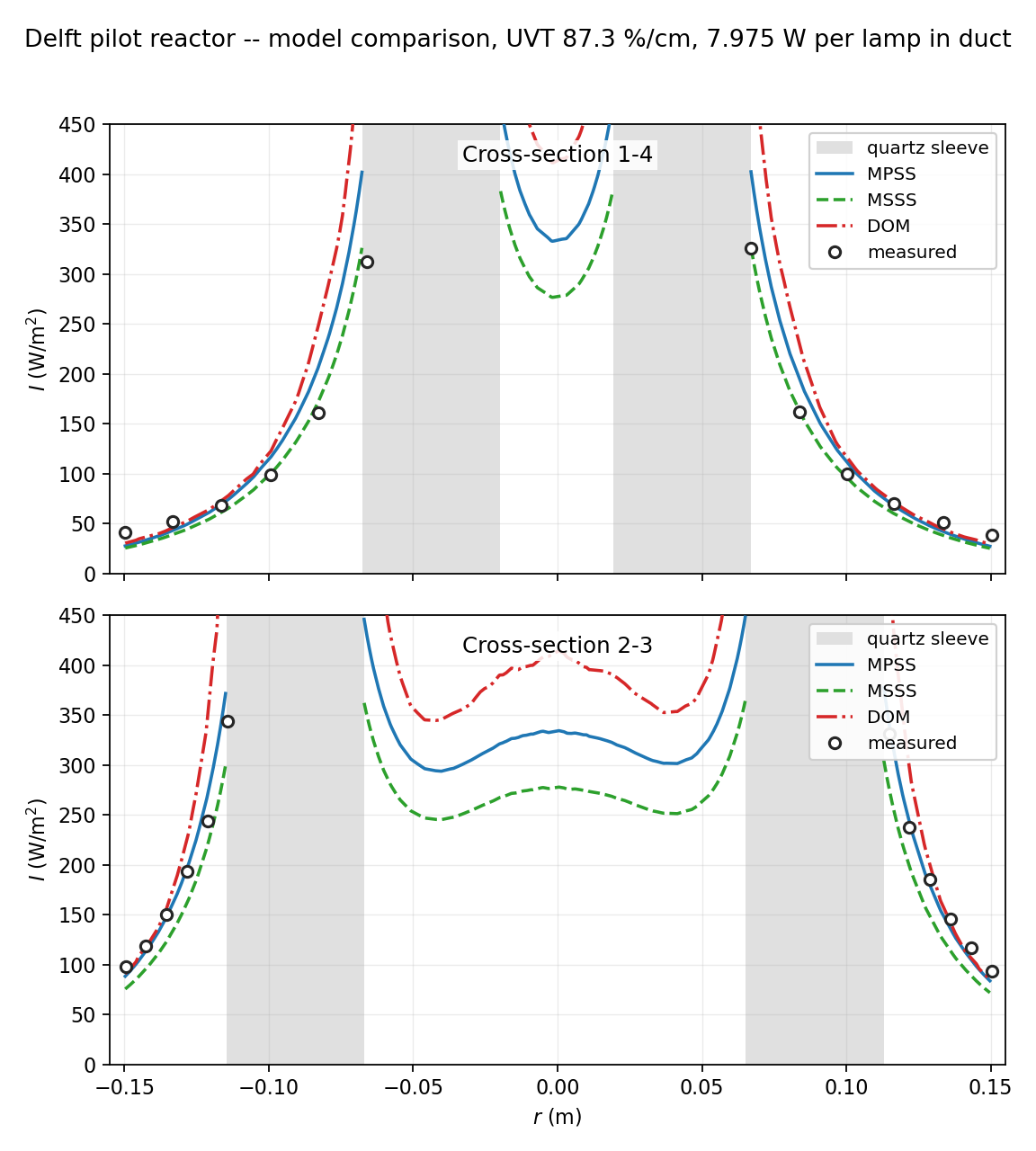
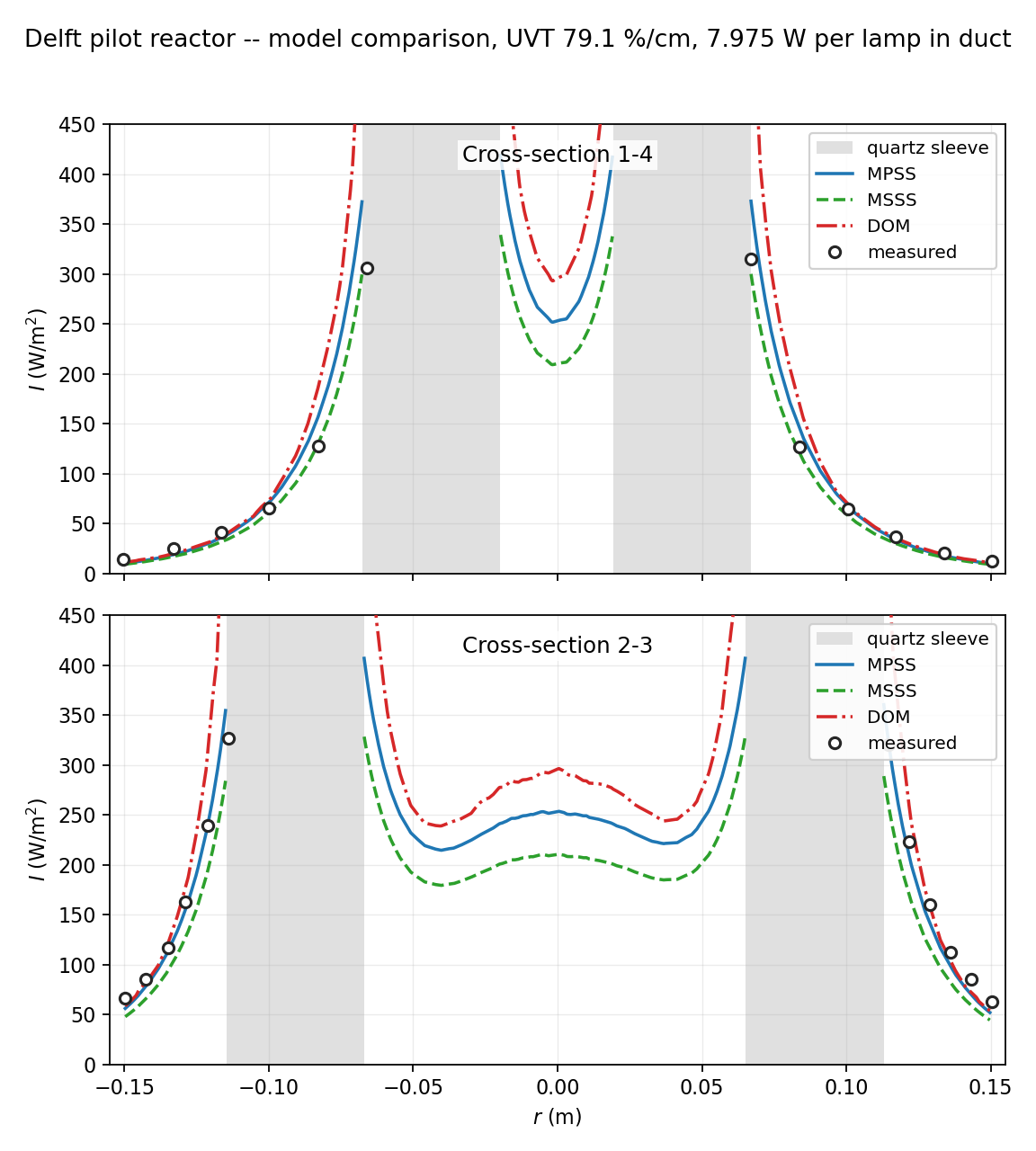
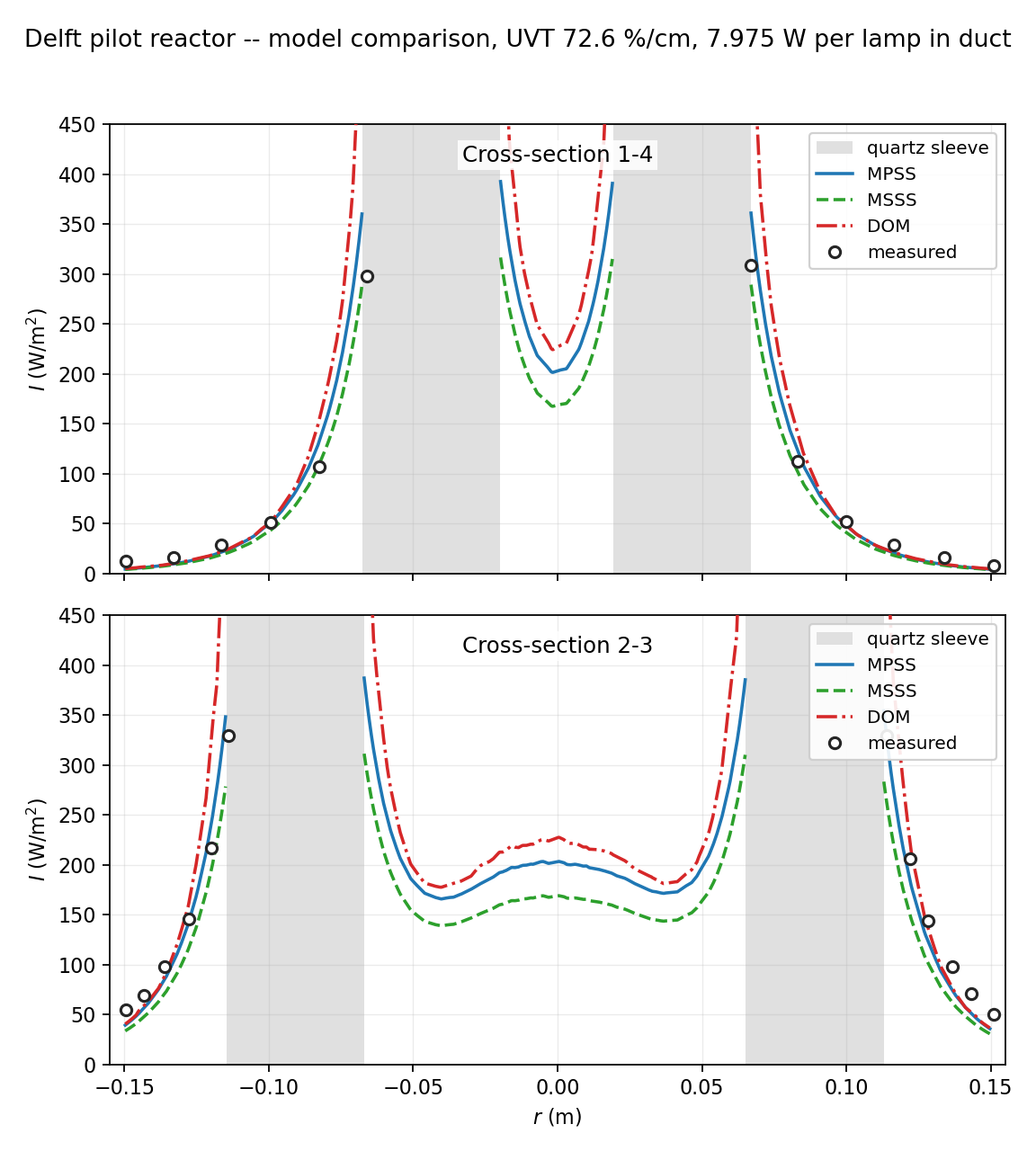
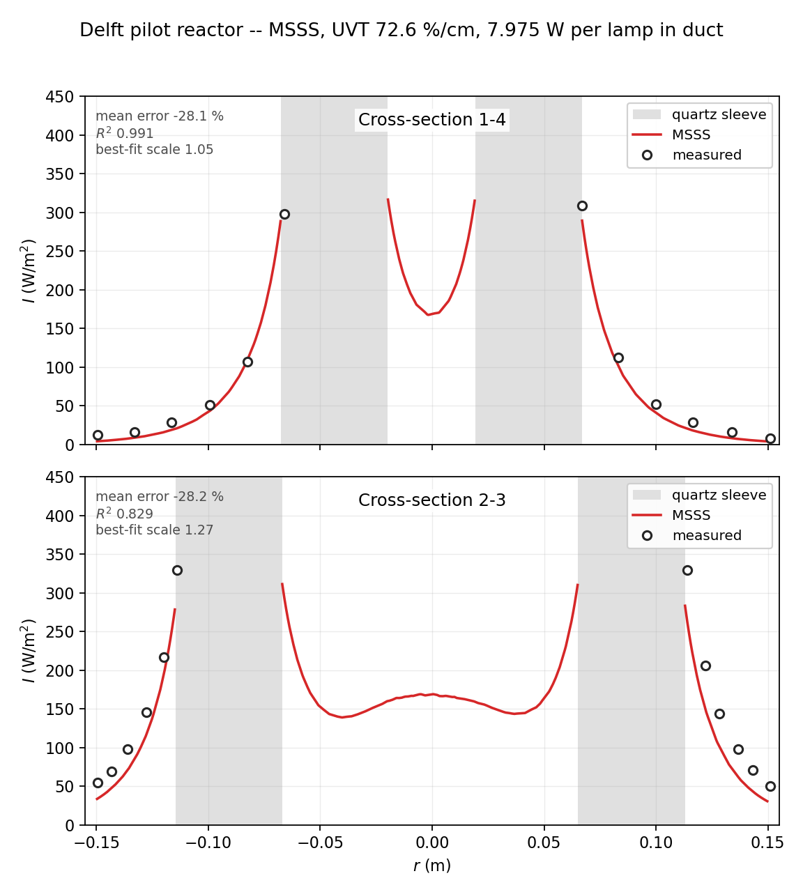
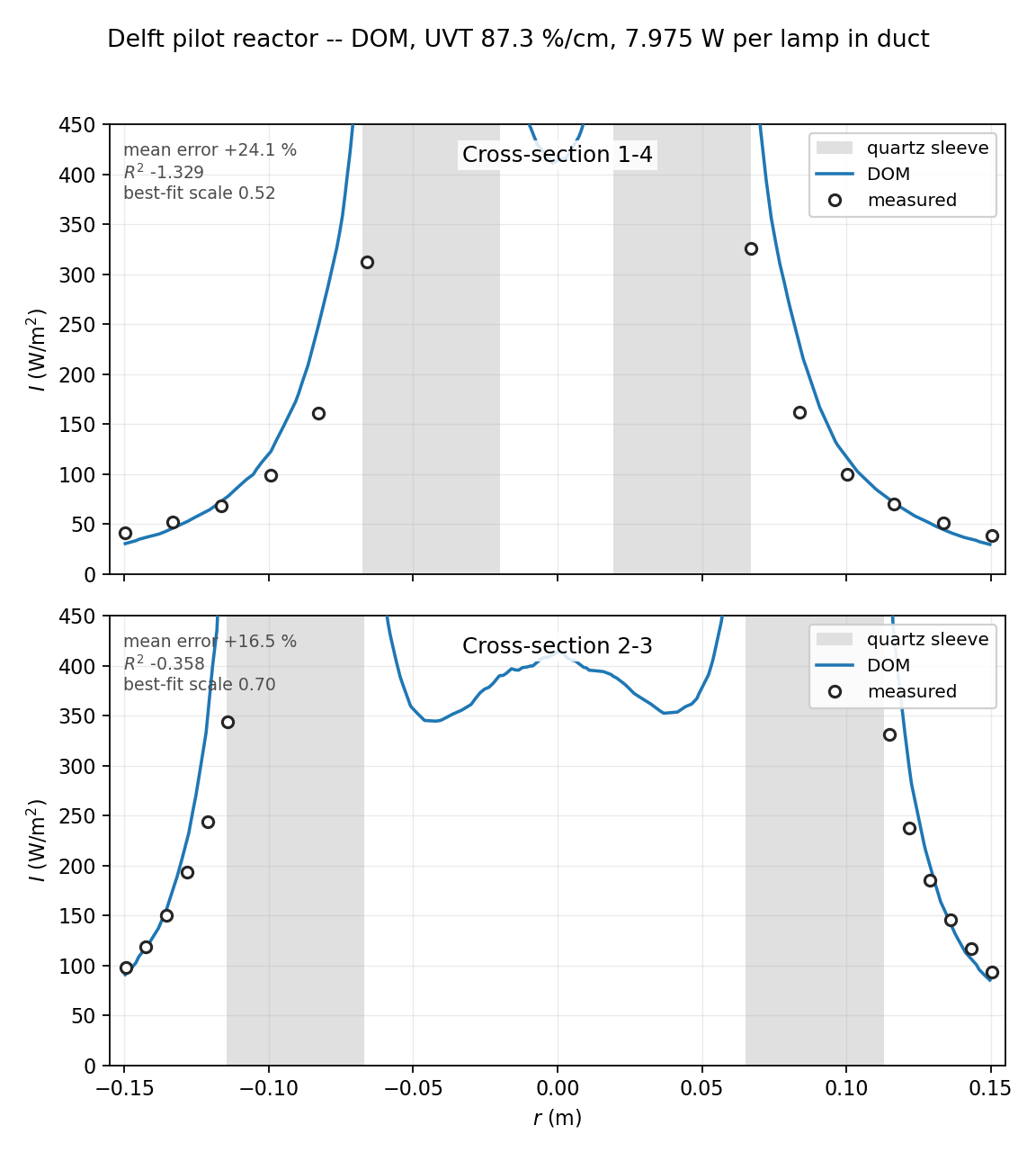
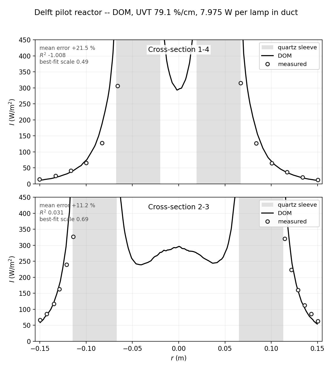
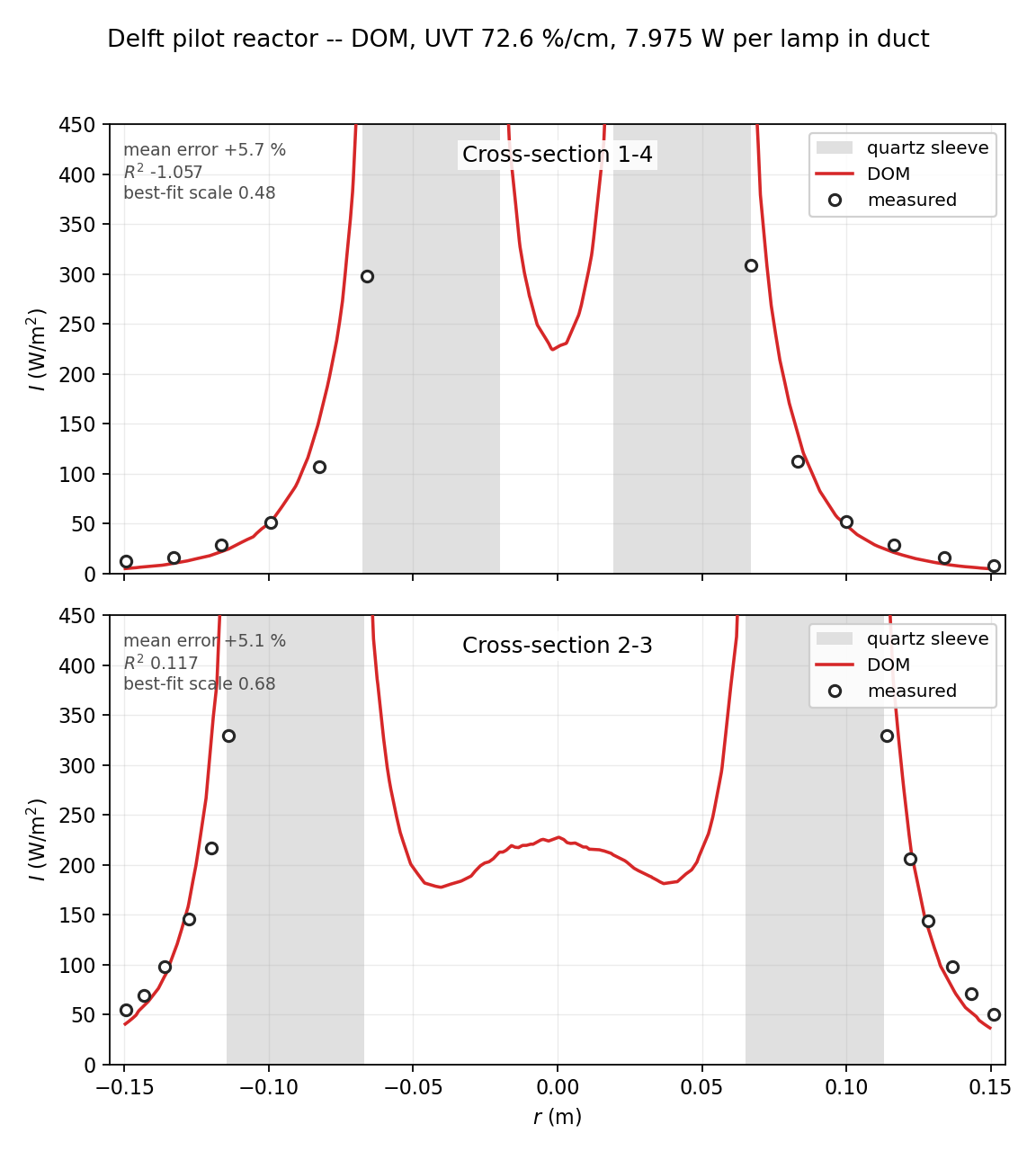
In the figures below, the gray band is the quartz sleeve the line passes through; fluence rate is undefined inside it since there is no water there. The curves diverge at the band edge because they are approaching the lamp surface, and the paper's original figures are likewise cut off at the same point.
Results — the three models against measurement
UVT 87.3 %
UVT 79.1 %
UVT 72.6 %
Statistics over 12 measurement points per line, two cross-sections × three UVT levels = 72 points in total. The multiplier is the lamp-power factor that minimizes the sum of squared errors — closer to 1.00 means the configured wattage is closer to correct, the same approach the paper used to arrive at 41 W.
| UVT | Model | Cross-section | Mean signed error | Mean absolute error | R² | Multiplier |
|---|---|---|---|---|---|---|
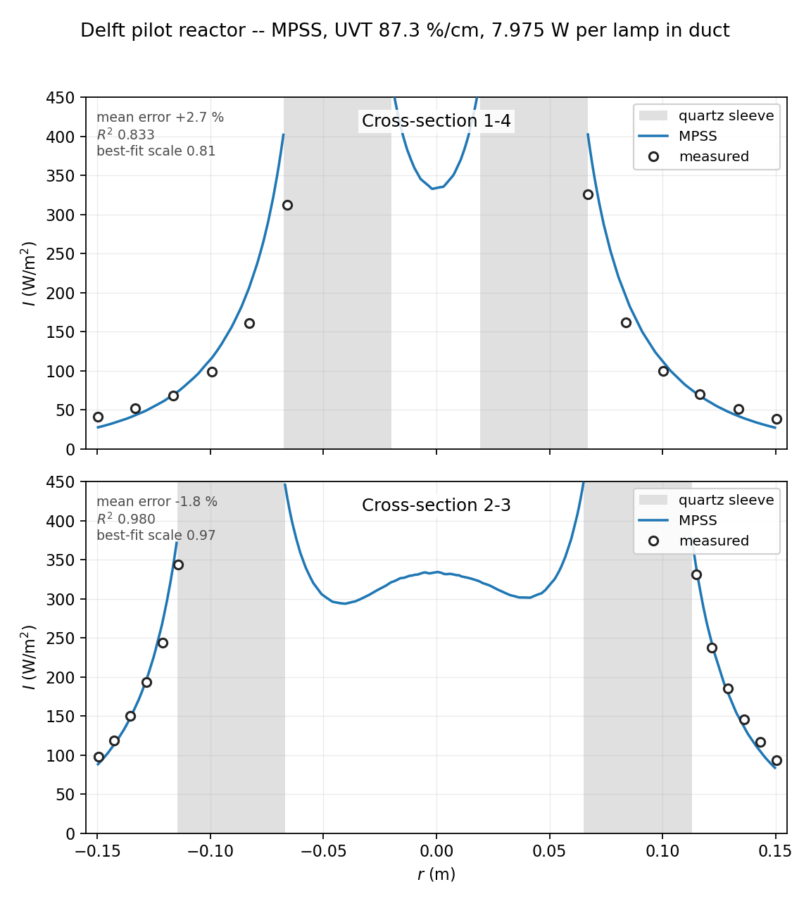
| 87.3 % | MPSS | 1-4 | +2.7 % | 19.5 % | 0.833 | 0.81 |
| 87.3 % | MPSS | 2-3 | −1.8 % | 5.7 % | 0.980 | 0.97 |
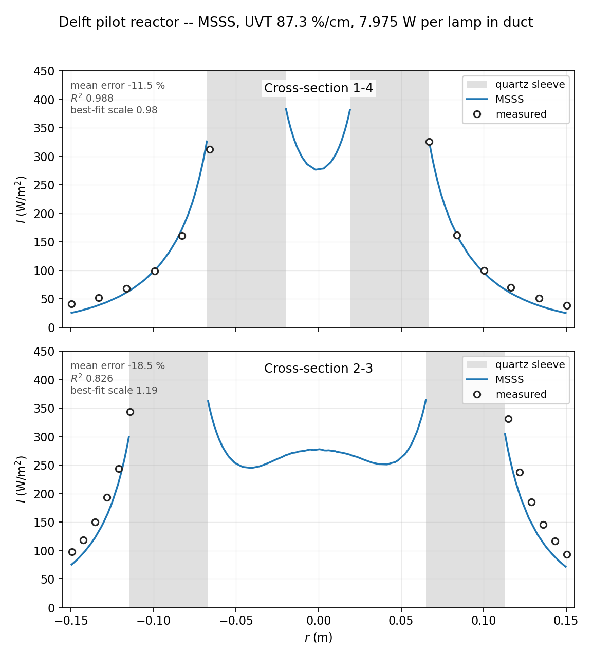
| 87.3 % | MSSS | 1-4 | −11.5 % | 13.7 % | 0.988 | 0.98 |
| 87.3 % | MSSS | 2-3 | −18.5 % | 18.5 % | 0.826 | 1.19 |
| 87.3 % | DOM | 1-4 | +24.1 % | 36.7 % | −1.329 | 0.52 |
| 87.3 % | DOM | 2-3 | +16.5 % | 20.8 % | −0.358 | 0.70 |
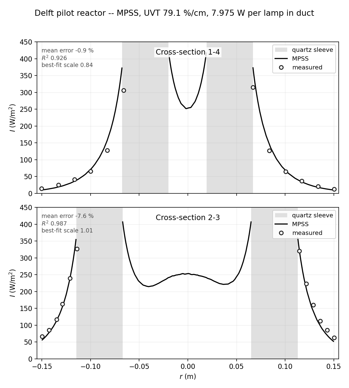
| 79.1 % | MPSS | 1-4 | −0.9 % | 16.5 % | 0.926 | 0.84 |
| 79.1 % | MPSS | 2-3 | −7.6 % | 8.5 % | 0.987 | 1.01 |
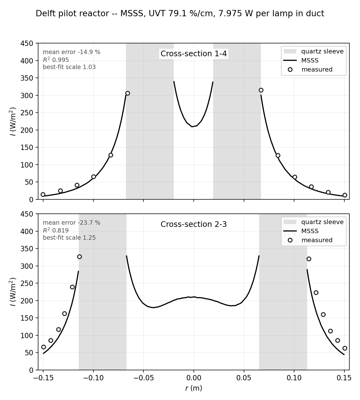
| 79.1 % | MSSS | 1-4 | −14.9 % | 14.9 % | 0.995 | 1.03 |
| 79.1 % | MSSS | 2-3 | −23.7 % | 23.7 % | 0.819 | 1.25 |
| 79.1 % | DOM | 1-4 | +21.5 % | 33.3 % | −1.008 | 0.49 |
| 79.1 % | DOM | 2-3 | +11.2 % | 19.7 % | 0.031 | 0.69 |
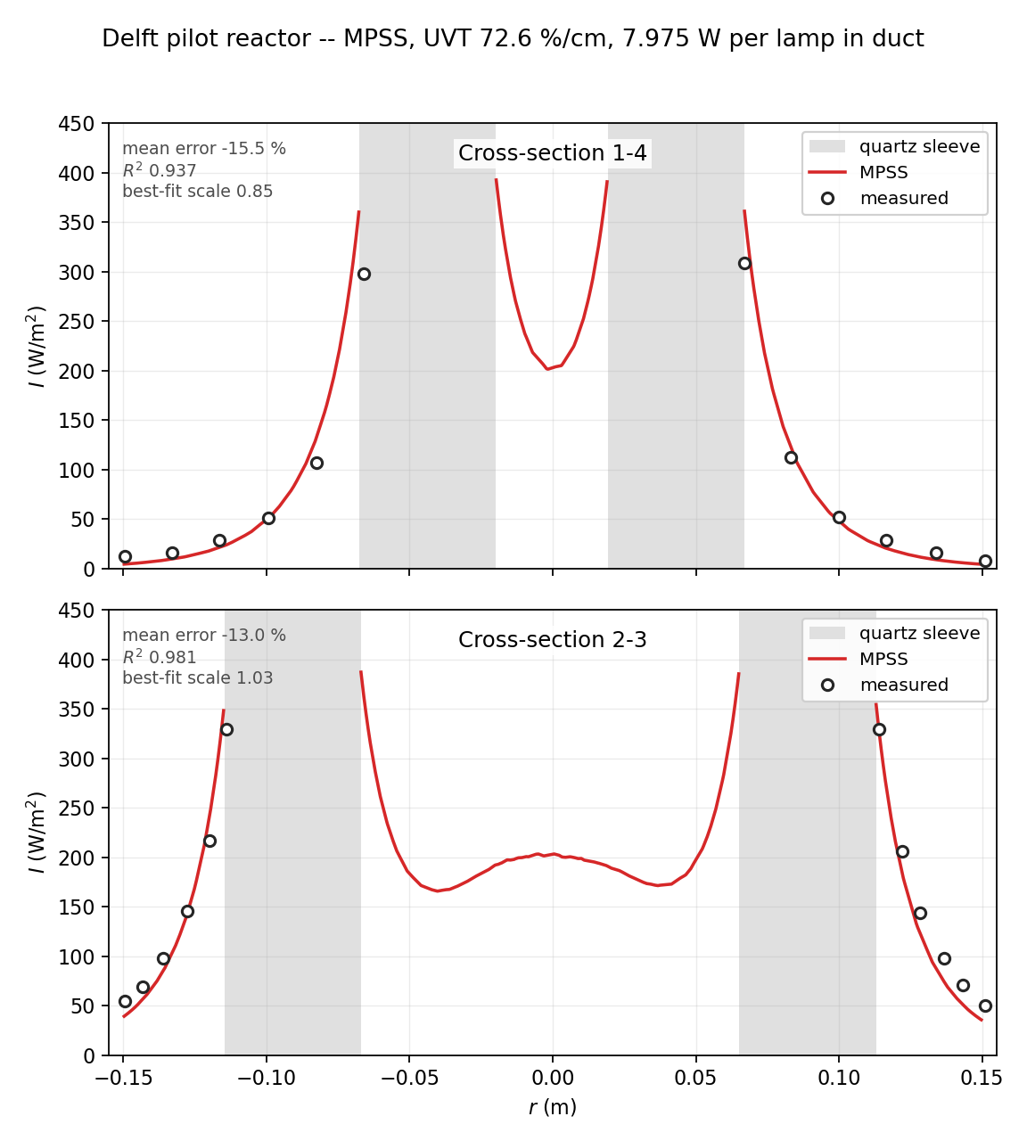
| 72.6 % | MPSS | 1-4 | −15.5 % | 27.6 % | 0.937 | 0.85 |
| 72.6 % | MPSS | 2-3 | −13.0 % | 13.7 % | 0.981 | 1.03 |
| 72.6 % | MSSS | 1-4 | −28.1 % | 28.3 % | 0.991 | 1.05 |
| 72.6 % | MSSS | 2-3 | −28.2 % | 28.2 % | 0.829 | 1.27 |
| 72.6 % | DOM | 1-4 | +5.7 % | 45.3 % | −1.057 | 0.48 |
| 72.6 % | DOM | 2-3 | +5.1 % | 25.6 % | 0.117 | 0.68 |
MPSS is the most accurate in absolute terms. At the outer cross-section, R² is 0.980–0.987 and the multiplier is 0.97–1.03, so the configured lamp power needs essentially no correction.
MSSS is the most accurate in shape. At the inner cross-section its R² of 0.988–0.995 is the highest of the three models. Its values run low overall, though, needing a multiplier of 1.0–1.27 to match magnitude — the same property seen in the in-air validation, where MSSS radiates π/4 of the total by definition (78.5 %).
DOM runs about 2× high near the lamps. A negative R² means it fits worse than a flat average line; the reason is explained separately below.
Per-model detail — variation with UVT
MPSS
MSSS
DOM
Why DOM runs high near the lamp
DOM represents the lamp as a surface source radiating diffusely from the sleeve's outer surface. Just outside a diffusely radiating surface, fluence rate is, by definition, twice the surface flux.
The computed result at the sleeve is 756 W/m², so DOM is consistent with its own boundary condition. The measurement at the same location is about 320 W/m². The solver is not wrong, then — the diffuse-surface boundary condition simply cannot represent the directional radiation passing through a refracting sleeve. MPSS and MSSS capture this because they compute Snell and Fresnel per ray.
This is not a numerical resolution issue
Checked by raising angular discretization 4× (128 → 512 directions). The two cross-section profiles moved by only −0.9 % / +0.1 % on average, and the optimal multiplier held to two decimal places (0.52 → 0.52, 0.70 → 0.70). This is a property of the model, not insufficient angular resolution.
This is the same phenomenon as DOM's +54.8 % at the 5 cm point in air, reported in the model comparison; the paper's authors likewise state that the DO model "significantly over-predicts the fluence rate near the lamp surface."
A trend common to all three models
As UVT decreases, all three models trend lower relative to measurement.
| Model (cross-section 2-3) | UVT 87.3 % | UVT 79.1 % | UVT 72.6 % |
|---|---|---|---|
| MPSS | −1.8 % | −7.6 % | −13.0 % |
| MSSS | −18.5 % | −23.7 % | −28.2 % |
| DOM | +16.5 % | +11.2 % | +5.1 % |
The three models take the lamp to be different things, but all handle attenuation with the same Beer-Lambert law. This shared shift, then, is not a property of any one model — it points to an input or physics the three share: the absorption coefficient itself, or the scattering and wall reflection that none of the three models represent. Direction is consistent too: stronger absorption reduces the direct beam, which increases the relative weight of those two terms.
From a design standpoint this is conservative. At low UVT the computed values run below measurement, so designing to those values means the actual dose will be higher than computed.
Which to use
| Purpose | Recommended model |
|---|---|
| Absolute fluence rate / dose in a multi-lamp reactor | MPSS — multiplier 0.97–1.03 in this case |
| Profile shape near the lamps | MSSS — R² 0.988–0.995 at the inner cross-section |
| Cases with scattering or wall reflection to account for | DOM — though it over-predicts near the lamp |
| Fast design iteration | MSSS (default) or MPSS |
In the in-air validation, MSSS was best near the lamp; in this reactor, MPSS is best in absolute terms. This is not a contradiction — the same underlying property, MSSS matching shape and MPSS matching magnitude, shows up differently in the two cases. In both documents, MSSS's multiplier runs above 1 and MPSS's stays close to 1.
The model is selected with solverConfig.radiationModel in the configuration file
("mpss" / "msss" / "dom"). All three models here were computed by changing only that one
line in the same configuration file.
Computational cost
Wall-clock time on the same grid (2.48 million cells), same machine, 4 threads.
| Model | Time | Notes |
|---|---|---|
| MPSS | 9 min 14 s | 1000 segments per lamp |
| MSSS | 9 min 18 s | same |
| DOM | 8 min 24 s – 9 min 35 s | 128 directions, converged in 16 iterations |
The three models cost about the same in this case, though for different reasons — MPSS and
MSSS scale as node count × lamp count × segment count, while DOM scales as
cell count × direction count × iteration count. DOM scales linearly with direction count, so
the 512-direction run used in the earlier validation took about 4× longer (a bit over 38
minutes).
Where the inputs come from
UVT reference path length — the paper states UVT as "%/cm," i.e. on a 10 mm basis. This matches the water-treatment field's standard convention (a 10 mm cuvette), and the reference path length is recorded in the configuration file as well.
Lamp power — the paper's Table 3 fits 41 W per lamp against its own measurements, and 41 W / 125 W (electrical) = 32.8 % is a typical UVC efficiency for a low-pressure lamp, so 41 W is the output of the whole lamp. The paper does not state the arc length, though, and since the reactor is 0.15 m deep, only 0.15 m of the arc is inside the reactor. The calculation used 7.975 W, the fraction of 41 W corresponding to an assumed arc length of 0.77 m (53 W/m).
The paper's own figures support this assumption. The 41 W curve sits near 320 W/m² close to the sleeve; putting all 41 W into just 0.15 m would put that point around 2300 W/m², off by an order of magnitude.
Reading the results when the lamp power is uncertain
Fluence rate is linear in lamp power. The
multipliercolumn above is the power factor that best fits measurement, so the relative comparison between models still holds even if the power assumption shifts. How the multiplier moves across the three UVT levels is more informative than its absolute value — a pure power error would stay constant across the three, whereas MSSS's multiplier moves 0.98 → 1.03 → 1.05.
Lamp positions — the lamp axis coordinates used in the calculation were back-fitted from the grid itself with a circle fit (residual ±3.5 µm, fitted diameter 0.047791 m against the paper's 0.0478 m). Two of the four lamps sit 1.0 mm and 1.9 mm off a symmetric layout, so using the grid's own values lets all three models be compared on exactly the same geometry.
The measured values were read from Figure 9 of the paper. The lamp specifications, reactor dimensions, and measurement positions are all in the published literature, so this comparison can be checked independently by a third party.
References
- Wols, B. A., Hofman-Caris, C. H. M., Harmsen, D. J. H., Beerendonk, E. F., van Dijk, J. C., & Chan, P. S. (2012). Comparison of CFD, biodosimetry and Lagrangian actinometry to assess UV reactor performance. Ozone: Science & Engineering, 34(2), 81–91.
- Liu, D., Ducoste, J., Jin, S., & Linden, K. (2004). Evaluation of alternative fluence rate distribution models. Journal of Water Supply: Research and Technology—AQUA, 53(6), 391–408.
- Bolton, J. R. (2000). Calculation of ultraviolet fluence rate distributions in an annular reactor: significance of refraction and reflection. Water Research, 34(13), 3315–3324.